How to Build a Lightweight Network SLA Monitoring Platform with Python

Network visibility isn’t just a nice-to-have; it’s essential for keeping operations running smoothly. Take, for instance, a network with multiple switches or routers installed across the facility, and physical access is tricky. If a remote node starts dropping packets or goes completely offline, your troubleshooting options quickly shrink to relying on ICMP alone unless you’ve got a unified network platform that gives you that kind of visibility.

In many industrial environments, managing this reality meant relying on raw terminal diagnostics. When an issue occurs on a remote segment, the immediate reaction is to fire up a continuous ping loop. But an infrastructure transit path is never a single, isolated point. Within an hour of troubleshooting a complex reachability issue, my desktop would transform into a chaotic grid of individual terminal tabs, forcing me to stare endlessly at scrolling text to manually track state changes.

This approach is inefficient and unsustainable in a production environment. Manual tab-gazing cannot reliably log long-term trends or capture transient network anomalies. If you step away from the desk for ten minutes, you lose the ability to answer the critical post-incident questions required during an operational review: When exactly did the path degradation begin? How long did the actual outage last?

This accountability deficit becomes even more glaring when dealing with upstream Internet Service Provider (ISP) links. When a primary circuit degrades, network teams often struggle to cleanly verify exactly when the service went down or mathematically prove whether the real-time latency failed to meet the average promised latency guaranteed in the provider’s SLA.

To eliminate this operational blindness and bring absolute empirical accountability to both internal links and external providers, I decided to build a lightweight network SLA monitoring platform from scratch. Using Python for low-overhead asynchronous polling and TimescaleDB for scale-ready time-series storage, I developed the Lightweight Network Monitoring Platform (LNMP). This architectural retrospective shares my thought process on building an event-driven software engine that turns raw ping behaviour into a reliable ledger for accurately calculating network uptime SLAs.

Minimalist Engineering

When creating a solution, there is sometimes the urge to over-engineer it. But I wanted a lean design centred on event-based data models, minimal footprint, reliable uptime, and simplicity as a top priority.

To achieve the absolute lowest overhead, I assembled a lean, native Linux architecture optimised for hardware-constrained environments. For the ingestion engine and backend, I chose Python utilising the FastAPI framework paired with native asyncio. This setup uses single-threaded, event-loop concurrency instead of resource-heavy multi-threading, enabling the daemon to poll hundreds of endpoints concurrently without waiting for sequential network timeouts to block execution threads. For the presentation layer, I used Vue.js because of its lightweight rendering and performance benefits, allowing me to build an interface focused strictly on historical investigation rather than real-time events. Finally, the data store uses TimescaleDB built on top of PostgreSQL. Instead of regular relational architectures that buckle under persistent logging, TimescaleDB automatically partitions metrics into time-series chunks, keeping query speeds instantaneous.

Initially, the planned feature list was expansive, including multi-protocol verification like TCP state checks, DNS resolution tests, and automated failure webhooks. But I had to focus purely on the two metrics that yield the highest diagnostic value for remote hardware: ICMP availability and latency tracking.

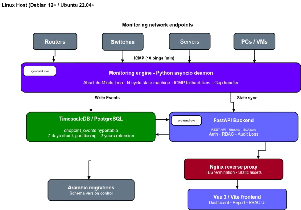
LNMP State Machine Flowchart

The 10-Ping Sub-Cycle and Dual-State Architecture

The first major architectural hurdle was data ingestion frequency. Storing high-frequency per-packet logging across hundreds of endpoints triggers significant table bloat and rapid row accumulation on disk. Conversely, standard tools that poll a single ping every 60 seconds suffer from a dangerous blind spot. If a transient patch of network jitter drops that single packet, the tool falsely logs a hard outage, creating rapid, artificial state flipping.

LNMP avoids this by running a high-fidelity sub-cycle of 10 pings inside each minute window, spacing the packets exactly 6 seconds apart.

$$\text{Ping Spacing} = \frac{60\text{ seconds}}{10\text{ packets}} = 6\text{ seconds per ping}$$

The metrics are calculated entirely in memory, writing only a single summarised row to the database every 60 seconds. To insulate the platform from packet-level flapping, I decoupled how the application classifies system health by introducing a dual-state architecture: detailed_state and operational_state.

Packet Success	Health Score	Detailed State	Operational State
10 / 10	100%	UP	UP
6–9 / 10	60% – 90%	UP-UNSTABLE	UP
1–5 / 10	10% – 50%	DOWN-UNSTABLE	DOWN
0 / 10	0%	DOWN	DOWN

The Detailed State tracks the raw per-minute truth, identifying if a link is perfect (UP), slightly dropping packets (UP-UNSTABLE), severely degraded (DOWN-UNSTABLE), or completely dead (DOWN). The Operational State normalises this data into a stable macro view. A link dropping 2 out of 10 pings is technically unstable, but it still passes production traffic; its operational state remains safely marked as UP, keeping long-term logs clean.

Simulating Chaos in the GNS3 Lab

Validating this edge-triggered logic required an environment capable of generating authentic network behaviour. In my GNS3 laboratory, I constructed a multi-hop transit path consisting of an R1, R2, and R3 routed chain.

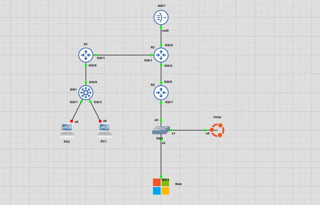
Multi-hop routed network path simulated inside GNS3.

The Ubuntu monitoring node running the lnmp daemon was positioned on a local segment connected to switch SW2, which sat directly behind router R3. This physical separation meant any checks directed at targets like PC1 or PC2 behind router R1 had to traverse multiple routed boundaries and navigate real-world network paths.

To suppress the inevitable link transitions and routing convergence delays inherent in this layout, the LNMP collection engine implements an in-memory N-cycle confirmation state machine, defaulting to a threshold of three consecutive cycles (N=3). When I simulated an interface flap or a route change on R2, the pending counters held the line entirely within volatile memory.

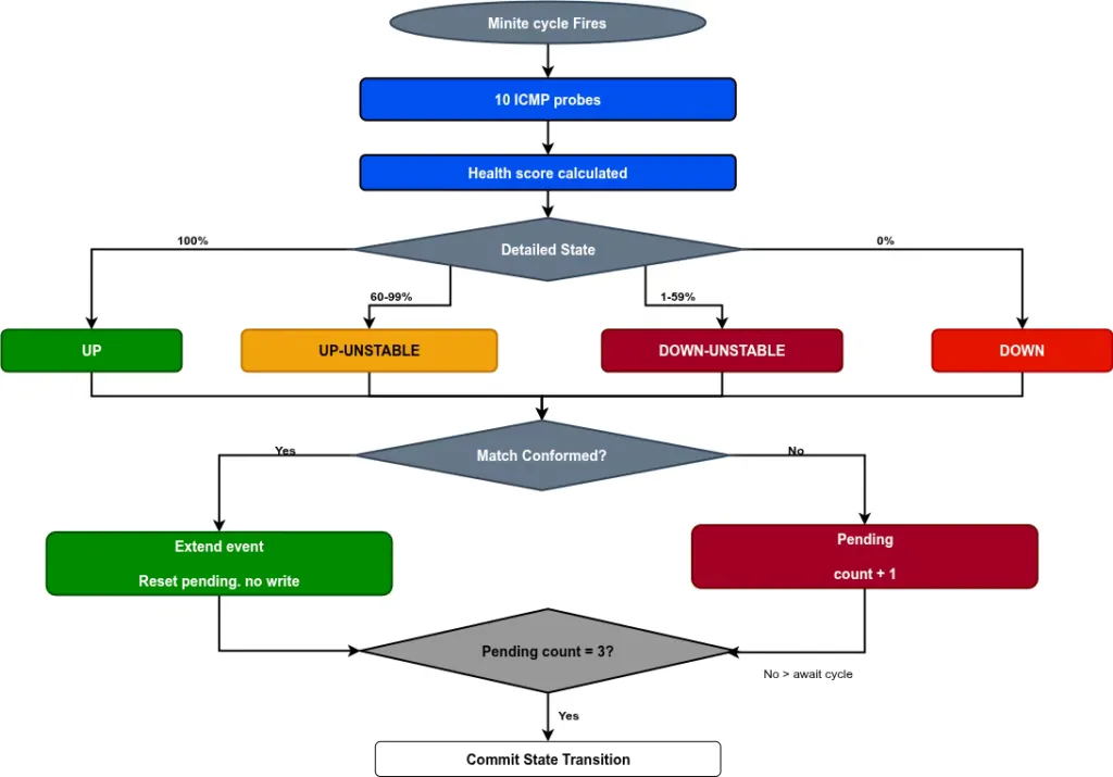
State Machine Flowchart.

Let’s look at the cycle-by-cycle confirmation flow during an outage event:

• Minute 1: The R2 link drops. PC1 returns 0 out of 10 successful pings. Detailed state switches to DOWN. Operational state remains UP. The pending status is set to DOWN with a count of 1. No database write occurs.
• Minute 2: The failure persists. Detailed state remains DOWN. Operational state remains UP. Pending count increments to 2.
• Minute 3: The third consecutive failed cycle is recorded. The pending count reaches the threshold of 3. The state machine officially commits the transition to the database, closing the long-running UP event and opening a new DOWN record.

By forcing the engine to evaluate 30 separate ICMP packets across a continuous 180-second window before committing a transition, the platform effectively eliminates alert fatigue. If a link flaps and recovers within a two-minute window, the counter resets instantly, sparing the database from processing lines of transactional noise.

How the Industry Tracks Availability

I believe it would give a lot of context to understand how the rest of the monitoring industry handles service-level data. Enterprise tracking methodologies generally fall into two broad architectural categories, both of which require significant manual effort to achieve basic mathematical accuracy.

SLA CALCULATION CATEGORIES

1. RAW TELEMETRY BUCKETS (Prometheus / Datadog)
   - Collects flat data streams continuously
   - Shifts the mathematical burden entirely to complex queries
-------------------------------------------------------------------
2. LEGACY RELATIONAL PLATFORMS (SolarWinds / Zabbix)
   - Relies on rigid relational tables
   - Requires manual admin toggles & strict maintenance windows
-------------------------------------------------------------------
3. NATIVE APPLICATION PRECALCULATION (LNMP)
    - Enforces window alignment & server gap filtering in core code
    - Delivers mathematically SLA metrics natively
-------------------------------------------------------------------

Category 1: The Raw Telemetry Bucket (Query-Time Manipulation)

Cloud-native tools like Prometheus and Datadog operate on a “collect everything, process later” philosophy. The underlying database is essentially a flat repository of timestamps and values. It possesses no native awareness of an endpoint’s deployment lifecycle or whether a sudden gap in data points signifies a crashed switch or a crashed monitoring server.

If you attempt to pull a monthly SLA percentage from a raw metric stream without modification, the calculation will be wildly inaccurate. To resolve this, these platforms shift the entire analytical burden onto the engineer at query time. The engineer needs to write complex database queries, like parsing PromQL range vectors, to handle missing data points and exclude time intervals from before the device was onboarded. If your dashboard query lacks these precise parameters, the system outputs distorted averages.

Category 2: Legacy Relational Platforms (Administrative Overhead)

Traditional enterprise suites like SolarWinds and Zabbix rely on structured database tables and relational mapping. These systems are capable of producing highly accurate historical records, but they demand constant administrative hand-holding to protect data integrity.

If your monitoring server requires a critical operating system patch or a routine reboot, you must remember to manually toggle all your monitored infrastructure nodes into an explicit “Unmanaged” or “Maintenance” state before pulling the plug. If you fail to perform this manual configuration, the database will aggressively log the server’s local downtime as a massive, simultaneous outage across all remote endpoints. The remote hardware takes an unfair performance penalty simply because the monitoring infrastructure went offline.

The SaaS Alternative and the WAN Boundary

Public SaaS utilities like Uptime Robot introduce a much cleaner, frictionless experience. For instance, Uptime Robot elegantly sidesteps the mid-month onboarding distortion by locking the evaluation timeline to the exact second a monitor is activated, ensuring prior historical gaps do not penalise the initial percentage.

However, SaaS tools poll exclusively on public cloud infrastructure. This makes them entirely useless for tracking nodes tucked safely behind an enterprise WAN boundary. You cannot monitor internal industrial networks or local server segments without exposing your internal infrastructure to the public internet through risky firewall modifications.

The Math of Truth: Lifespan Alignment and Honest SLA Calculation

To ensure complete analytical integrity without making you write complex database queries every time you access a dashboard or manually set maintenance windows before a server reboot, LNMP integrates these fixes directly into the application layer. It natively tracks internal server outages through the monitoring_service_events and automatically enforces lifespan alignment right out of the box.

First, the engine establishes an effective time window by matching your query boundaries against the exact moment the endpoint was onboarded. Let $S$ represent your query start time, $E$ represent the query end time, $C$ represent the endpoint’s creation timestamp, and $N$ represent the current system time. The engine defines the effective start and end boundaries through two simple comparisons:

$$S_{\text{eff}} = \max(S, C)$$

In plain terms, the system ensures your reporting window never starts before the device actually exists in the database.

$$E_{\text{eff}} = \min(E, N)$$

In plain terms, the window cannot extend past the present moment into an unmonitored future.

From these boundaries, the total elapsed lifespan seconds are calculated cleanly:

$$T_{\text{total}} = \max(0, E_{\text{eff}} - S_{\text{eff}})$$

In plain terms, this isolates the exact number of seconds the device has spent registered within your selected report window.

The second major optimisation handles the “Unknown State” caused by server blackouts. If the monitoring engine goes offline for a reboot or a database migration, it cannot collect telemetry. LNMP tracks these internal application gaps $U$ in a dedicated infrastructure table. To calculate an honest SLA denominator, the engine subtracts those unknown blackout seconds from the total elapsed lifespan:

$$D_{\text{sla}} = T_{\text{total}} - U$$

In plain terms, your baseline window only includes the time the monitoring engine was actually online and capable of observing the network.

To see this math in action, consider a concrete example. Suppose a remote switch was registered 30 days ago, and your query window covers that entire 30-day period. If the monitoring server was offline for 2 hours due to an internal software upgrade, LNMP sets your true SLA denominator to 30 days minus 2 hours, rather than a full, uncorrected 30 days. This means the 2 hours of missing data are completely neutralised.

Finally, the availability percentage ($A$) is derived using a streamlined conceptual equation:

$$A = \left( \frac{\text{Uptime Seconds}}{D_{\text{sla}}} \right) \times 100$$

In plain terms, you divide the confirmed seconds spent in an operational UP state by your corrected monitoring window, multiplying by 100 to yield a percentage. Behind the scenes, the source code runs safety checks to enforce a strict 0% to 100% boundary and automatically rounds the final output to two decimal places, delivering a visually clean and mathematically sound uptime report.

Turning Domain Modelling into Scale-Ready Storage

Database architecture for a high-frequency event recorder is fundamentally about mapping data lifecycles to physical constraints. To keep the storage layer clear and accessible, I worked through the core parameters to map the system entities into four highly optimised tables:

• endpoints: Houses the asset source of truth, utilising native INET Types for IP tracking and implementing a soft-deletion flag so historical availability metrics remain intact when a device is retired.
• endpoint_events: The primary hypertable managed by TimescaleDB, storing state transitions and partitioned automatically by the start_time
• monitoring_service_events: Logs internal application gaps, providing the exact blackout metrics required by the SLA calculator.
• users and roles: Enforces role-based administrative boundaries using secure password hashing and clean key mappings.

The time-series optimisation occurs within the endpoint_events. To maximise read performance across a multi-year retention window, I applied a targeted composite index:

SQL

CREATE INDEX idxendpointeventsincidentquery
ON endpointevents (endpointid, operationalstate, starttime DESC);

When an operator requests an uptime summary panel or a historical trend chart, this index allows the PostgreSQL engine to run a rapid index-only scan. It isolates the exact endpoint and its operational history in milliseconds, completely bypassing the need to perform an expensive full-table scan across thousands of unrelated records.

Accelerating Schema Design and Boilerplate with Antigravity

This project was a true exercise in what modern developers call vibe coding. Coming from a traditional network engineering background, stepping into full-stack development meant facing a daunting wall of boilerplate code, asynchronous database connections, and frontend components. To accelerate this implementation, I utilised the AI programming companion, Antigravity.

The speed at which Antigravity scaffolded the initial framework was incredible. It spun up clean FastAPI routers, established the Vue 3 component architecture, and handled the iterative design of our tables with ease.

I spent hours refining the schema parameters, using Antigravity to rapidly iterate on table structures until the design was minimal, efficient, and completely transparent to troubleshoot. We stripped out unnecessary variables until the configuration layer was perfectly lean.

However, it is vital to document exactly where the magic hits the wall. Antigravity was exceptional at structural boilerplate, but it completely faltered when confronted with low-level infrastructure constraints. It routinely struggled with the syntax required for unprivileged Linux network sockets, regular expression parsing for system ping fallbacks, and microsecond-level timing loops. The edge-triggered logic of the state machine and the precise time-series boundaries required rigorous manual intervention, code refactoring, and verification inside the laboratory environment.

Why Less is More

When reviewing the final architecture of LNMP, the features left out are just as important as the features built. The project brief originally included advanced concepts like Quality of Service (QoS) analysis, automated traceroute diagnostics, and deep service quality streaming telemetry. However, early in the design phase, a deliberate decision was made to aggressively reduce the scope.

The objective was never to build a replacement for mature, feature-heavy monitoring ecosystems. Those platforms excel at broad, multi-layered observability, but they are often operationally heavy, difficult to customise, and resource-intensive for small or distributed environments. By narrowing the scope down specifically to ICMP availability, endpoint management, and historical outage analytics, the project minimised immediate implementation risk while maximising core architectural reliability.

Because simplicity was prioritised over feature count, the system gained immediate operational efficiencies. For instance, because the event-based engine stores state transitions instead of raw, high-frequency ping telemetry, the storage footprint drops dramatically.

With a stable, predictable foundation established, a clear roadmap can be laid out for future versions without drowning in technical debt:

• Automated Diagnostics: Triggering automated, hop-by-hop traceroute diagnostics the exact moment a DOWN state transition is confirmed, capturing the precise path failure before routing tables reconverge.
• Proactive Alerting: Integrating a lightweight webhook and notification engine to instantly alert operators of verified state changes.
• Real-Time Dashboards: Introducing WebSocket streaming support to turn the reporting UI into a live NOC monitoring portal.
• Distributed Scalability: Implementing multi-node orchestration to allow centrally managed, distributed polling engines to feed a unified database tier.

Conclusion: Building to Learn

Building LNMP was an invaluable reminder that the most effective way to understand application architecture is to engineer your way through your own daily operational constraints. What began as a personal itch to clear a chaotic grid of terminal windows from my workstation ultimately evolved into a lean, scale-ready uptime analytics platform.

Taking this project from a loose collection of ideas to a functioning time-series system forced me to step completely outside my comfort zone as a network practitioner. It made me grapple directly with edge-triggered state transitions, data ingestion strategies, and the subtle mathematical differences between raw metrics and objective truth. The platform does not try to compete with massive enterprise monitoring suites, but it achieves exactly what I set out to discover: it proves that you can build a lightweight, highly accurate internal tool that remains entirely understandable and maintainable over long retention windows.

• The complete open-source codebase for the polling daemon, backend API, and interface dashboard is available on GitHub: https://github.com/dc8official/lnmp.git